
Continuing my exploration of basic image processing I've set about modifying the contrast within an image. This has proven to be more of a challenge than I first anticipated — which is fun!
It has proven challenging to find a satisfying description of contrast. I've learned quite a bit about how it can be defined mathematically, or visualized, but the closest plain-english description comes from Wikipedia:
Contrast is the difference in luminance or colour that makes an object … distinguishable.
These lecture notes from an electrical engineering lecture at NYU proved both helpful and interesting, especially for pointing me to the term histogram equalization.
I've allowed myself to work only in greyscale here, after reading the contrast enhancement lecture notes linked above. It appears to be fundamentally similar for color images (except you modify each of the three RGB values independently). Because I'm still getting my feet wet, I think getting something working in greyscale is sufficiently interesting.
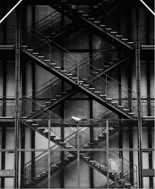
Once again, I'm working with a modified image, taken from Matt Seymour (I detailed previously how I achieved a greyscale effect based on the luminance values of each pixel):
(require 2htdp/image (except-in plot line))  ;; avoiding an import collision
(require math/statistics)
(define sample-image (bitmap/file "stairs.jpg"))

(define (luminance-lst image)
  (for/list ([value (image->color-list image)])
    (luminance value)))
I've defined a function to construct a list of the luminance values (based on the luminance function from the previous post). This is an easy shorthand for the grey values because each grey is a triple of the luminance.
(define (counter value-lst)
    (define hash-counter (make-hash))
    (for/list ([color value-lst])
      (hash-update! hash-counter color add1 0))
  hash-counter)

(define counts (counter (luminance-lst sample-image)))
(define kv-list (for/list ([key (hash-keys counts)])
                  (vector key (hash-ref counts key))))
With a list of some 300,000 pixels, it becomes important to define an aggregate data structure, here I'm calling it a counter, but it is just a hash table of grey values for keys and a count of incidents of those values in the image. I've since found there is a built-in function for this sort of thing, but mine is specific to the immediate next step, so I'll be using my own.
(plot
   (discrete-histogram
    (sort kv-list < #:key (lambda (v) (vector-ref v 0)))))
Here I'm sorting based on the first value (the luminance) in the
kv-list of grey-counts:

An alternative view of the same histogram information is a cumulative distribution of the values. For the case of an equalized histogram, the distribution should be a line with a constant slope because each "step" contributes an equal amount to the total.
I have to be honest, I lost a bit of patience here and the code quality probably shows it, I've resorted to writing some unidiomatic, less-than-optimal code to hack together a cumulative distribution tracking:
(define (distribution sorted-list)
  (define prior 0)
  (for/list ([item sorted-list])
    (define current (/ (vector-ref item 1) pixel-count))
    (define new-value (+ current prior))
    (set! prior new-value)
    (vector (vector-ref item 0) new-value)))
Using the sorted list of grey-values, I'm re-making a new list of the sum of the current grey-value pixels and all those prior (where "prior" implies those grey-values "less than" the current). The dotted line represented what the distribution of an ideally equalized histogram would be.

From this, it is obvious that approximately the first 12% and the last 30% contribute little to the picture, meaning the number of both darks and lights will be increased when we equalize the histogram, at the "expense" of those values visible as a spike around the 12-15% range.
After reading this explanation from UCI on histogram equalization I came up with the formulation below:
(define look-up-table (make-hash))
(for ([item sorted-grey-list]
      [multiplier (distribution sorted-grey-list)])
  (hash-set! look-up-table (vector-ref item 0)
                           (* (vector-ref item 0) (vector-ref multiplier 1))))

(define (transform-grey color)
  (define modified-grey (floor (hash-ref look-up-table (grey-value color))))
  (make-color modified-grey modified-grey modified-grey))
The key realization for me was that I couldn't devise a pure function
to calculate the individual adjustments per grey-value without first
computing the distribution for each of the 256 possible values
(0x00-0xFF). With that in mind, I've created a hashmap relating
the grey value and what I term a multiplier, with which to adjust the
value.
The formula is, in effect:
(number of occurrences of a particular grey)
 ------------------------------------------   X  (value of the particular grey, 0-255)
            (number of pixels)
This can be mapped across the original greyscale image to modify each pixel in turn:
(define (create-bitmap transform img)
  (color-list->bitmap
   (transform img)
   (image-width img)
   (image-height img)))

(create-bitmap (lambda (img)
                 (map transform-grey (greyscale img)))
               sample-image)


I should perhaps not be surprised that the result is imperfect. The histogram reveals that the relative difference has been equalized some, but not entirely. Similarly, the cumulative distribution shows a favoring of the darker tones (I think) in the resulting image. I think this was actually called out in lecture notes from NYU — we can't get a perfectly flat histogram with a discrete implementation. I'm quite pleased with the result though and I'm downright astonished that things more or less worked as I intended after just a bit of reading on the image processing.