Ray Tracing in J

I've been reading up on J and decided another small project was in order, this time I've written a minimal ray tracer.

Brevity

J is, perhaps infamously, a terse language. I think it may sometimes get unfairly discounted for this brevity because of the flavor of the syntax (namely, ASCII). It can be a little hard to describe, but the syntax isn't the hard part of learning J, the jarring parts are a result of the paradigm differences in array programming. By the time I've started to wrap my head around the very functional, array oriented style of programming the syntax has started to fall away. At least in the case of my own code I don't find the syntax being an obstacle, I'm curious how this would hold up in the face of someone else's code.

Tacit Verbs

One piece of syntax that bears explaining is J's means of tacit programming (that is, functions which make no reference to their arguments). While there is a bit more depth to it than I bother using, I've limited myself to using mostly trains of three verbs, so-called forks. A fork is a function comprised of three verbs, F G and H and might look like this:

myNewVerb=. F G H    NB. results in application (F(y)) G (H(y))

The parsing rules for J identify this pattern and apply the function in a specific way; the canonical example is to define "average":

sum=. +/
divide=. %
count=. #
average=. sum divide count

If you applied it to an array 1 2 3 4 5:

average 1 2 3 4 5
NB. (sum 1 2 3 4 5) divide (count 1 2 3 4 5)

One last thing that may confuse the untrained eye is the order of evaluation. Sentences respect the traditional means of evaluating parenthesized phrases first, but otherwise proceed from right to left. An example:

   - +/ 1 2 3
_6

The result will be the sum of 1 2 3 (6), which is then negated, so the result is -6 (which is written as _6 to avoid confusion with the minus/negate symbol).

Utility Verbs

I've written several verbs in the tacit style that are generally useful or improve the reading of the program, even when they're only used once. The first is magnitude, which returns the magnitude of a vector:

magnitude=: [: %: [: +/ *:      NB. sqrt of sum of squares

The comment should suffice for those who don't yet know the syntax of J but it may be worth pointing out two interesting details. The first is the fact that this "train" looks like it is 5 verbs, which doesn't sound like a fork at first. The thing to keep in mind is that forks can compose on top of other forks, so this may be viewed like:

• [: %: [: +/ *: a train of 5 verbs
• [: %: ([: +/ *:) the first fork is parenthesized
• the second fork is now F G H, where H is the parenthesized fork
• the resulting application is like ([: y) %: (([: +/ *:) y)

The use of [: is a little weird to understand, but it is basically a no-operation left argument to ensure that the verb is evaluated as a function of one argument instead of two. This is a consequence of J's overloading of verbs for the two cases, e.g. 3 % 4 is "3 divided by 4", but % 4 is "reciprocal of 4". By using [: in a train we ensure that whatever is left of % isn't taken as a left argument and instead we use the monadic form of the verb.

Although it isn't used much here, one thing that is really attractive about array programming is the way verbs can operate independent of dimensionality. Here I take the magnitude of a two-dimensional vector and then a three-dimensional vector (which is what I use throughout the ray tracer):

   magnitude 6 8
10

   magnitude 3 4 12
13

normalize=: ] * [: % magnitude  NB. scale by reciprocal of magnitude
dotproduct=: +/ . *

Both normalize and dot product aren't particularly interesting, normalize is notable for composing a new verb train from the previously defined magnitude without any special syntax or handling.

toRGB=: ([: <.&255 >.&0) & ([: <. 255&*) NB. 0->1 becomes 0->255 (clamped)

Throughout the ray tracer I deal with color as vectors of 3 floating point numbers, intended to be between 0 and 1.0. In order to map the range into the RGB space I'm doing max(0, min(floor(x * 255), 255)). & ("bond") is used to partially apply arguments to a verb, a simple example would be to define "addOne" as +&1. Interestingly, & can bond nouns to verbs to apply arguments but it may also be used to compose functions as in math, e.g. (f ∘ g)(x) = f(g(x)) is analogous to f&g y (eliding a few details here).

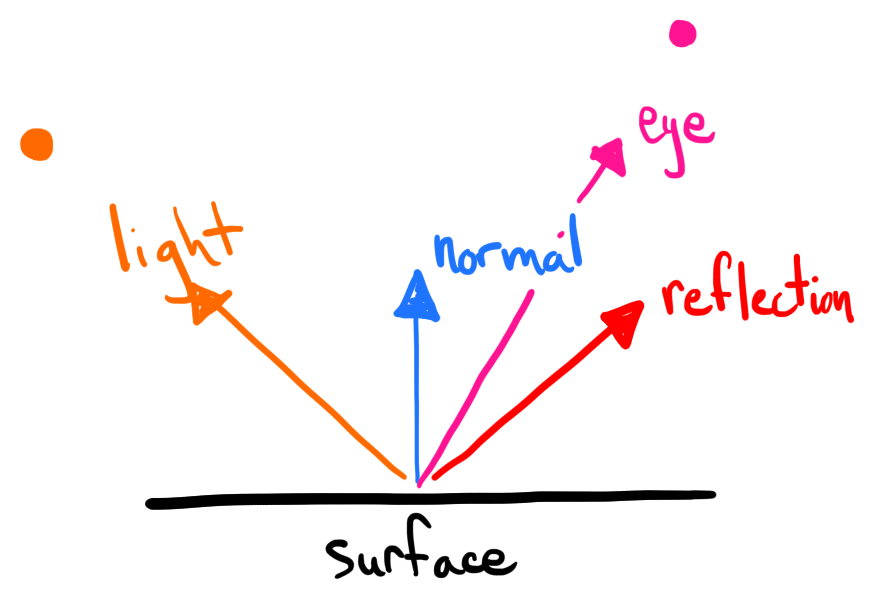
Reflection is defined as a verb taking two argument, a vector and a normal. It works by subtracting the vector and the normal scaled by twice the dot product of the vector and the normal.

reflect=: [ - ] * +:@dotproduct          NB. (vector normal)

Given an array of intersections (defined later) a "hit" is defined as the smallest positive intersection. This identifies which of the points the ray "touches" are to be drawn, since the vector "moves" in the time dimension it means we pick the first contact of the ray with the sphere:

hit=: ([: {. /:~) & (0&< # ])   NB. smallest positive intersection

It is a little interesting due to the way the filter works as part of the first train (0&< # ]). The predicate (F) is defined as < (greater than) bonded (&) with 0, the right-most verb (H) is simply right-argument (]) and doesn't do anything but return the argument supplied to it. Finally these two are combined with copy (#), the verb G in the train so that an application looks like this:

0&< # ]    NB. F G H
(0&< # ]) 3 6 0 8 1 0    NB. applied to an array y
(0&< y) # (] y)    NB. turns into (F(y)) G (H(y))
(1 1 0 1 1 0) # (3 6 0 8 1 0)    NB. copy uses a boolean array
                                 NB. to decide which to copy
3 6 8 1

From there I just sort ascending (/:~) and take the first item ({.).

Non-Tacit Verbs

While the tacit "utility" verbs I've defined are (at least to me) interesting in their own right, the remaining pieces of the ray tracer don't lend themselves to similar definition. It is entirely seamless to switch to explicit verb definitions where they make more sense, here in the case of defining intersect:

intersect=: dyad define         NB. (origin direction)
a=. y dotproduct y
b=. 2 * y dotproduct x
c=. (x dotproduct x) - 1
discriminant=. (*: b) - (4 * a * c)
if. discriminant >: 0 do.
  i1=. ((- b) - (%: discriminant)) % +: a
  i2=. ((- b) + (%: discriminant)) % +: a
  i1 ; i2
else.
  0                             NB. lest we return the last calculated value...
end.
)

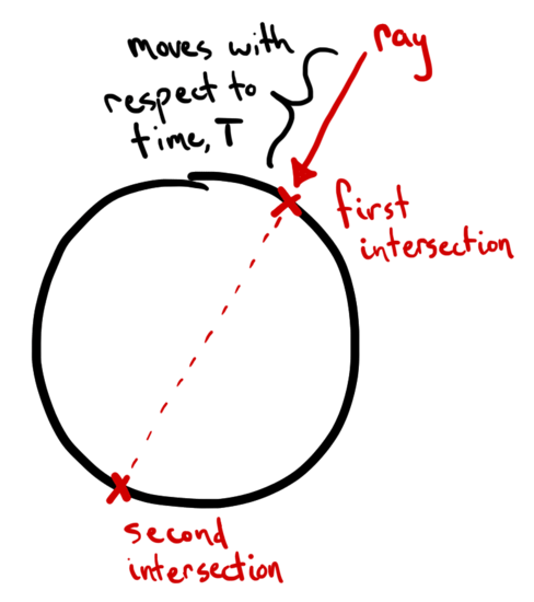
The definition for the intersection is pretty much straight out of a textbook and J really shines in a nearly direct translation. The one oddity I added was to return 0 in the case of a discriminant (b²-4ac) less than 0, this allows me to modify the behavior later in the program when coloring pixels based on the time of intersection.

Thus far all of my verbs have taken only 1 or 2 arguments, as is usual for J verbs. There are occasions where it is too onerous to write everything in this way, such was the case for rendering the lighting of a point. It really needs a number of pieces of information, some of them composite, J supports this with a kind of argument unpacking seen here on lines 2-4:

lighting=: monad define
'light material position eye normal'=. y
'lPosition lIntensity'=. light
'mAmbient mDiffuse mSpecular mShiny mColor'=. material
effectiveColor=. mColor * lIntensity
ambient=. effectiveColor * mAmbient
lightv=. normalize lPosition - position
l=. lightv dotproduct normal
r=. ((- lightv) reflect normal) dotproduct eye
diffuse=. (l>:0) { > (0 0 0) ; l * effectiveColor * mDiffuse
specular=. (r>:0) { > (0 0 0) ; lIntensity * mSpecular * r ^ mShiny
ambient + diffuse + specular
)

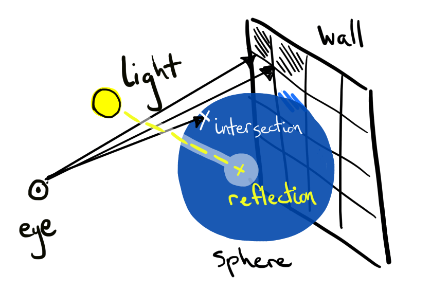
In order to "drive" the program there's one important bit left to write. It'll be responsible for sizing an area to "draw" onto, along with a small bit of math to orient the "eye" to the scene and define our light source and material:

trace=: dyad define             NB. (width (x y))
'xcoord ycoord'=. y
rOrigin=. 0 0 _5
wallZ=. 10
wallSize=. 7.0
pixelSize=. wallSize % x
position=. ((- -: wallSize) + pixelSize * xcoord) , ((-: wallSize) - pixelSize * ycoord) , wallZ
rDirection=. normalize position - rOrigin
contactTime=. hit >rOrigin intersect rDirection
if. contactTime do.
  pos=. rOrigin + rDirection * contactTime
  normal=. normalize pos
  eye=. -rDirection
  light=. (_10 _8 _10); (1 1 1) NB. position intensity
  material=. 0.1 ; 0.9 ; 0.9 ; 200 ; 0.5 0.2 1 NB. ambient diffuse specular shiny color
  lighting light; material ; pos; eye; normal
else.
  0 0 0
end.
)

This verb takes two arguments, one of them compound, the first is a "canvas" size, only square images are supported; the second is a single x, y position. Because trace takes a single x, y position I need an array of all the coordinates of the "canvas", for that I define:

coordinates=: [: (] ,"0 |:) 2&# $ ] # i. NB. y is square array width

This is another tacit verb of multiple forks, it isn't particularly interesting but boxing the result reveals the work it is accomplishing:

   <"1 coordinates 5
┌───┬───┬───┬───┬───┐
│0 0│0 1│0 2│0 3│0 4│
├───┼───┼───┼───┼───┤
│1 0│1 1│1 2│1 3│1 4│
├───┼───┼───┼───┼───┤
│2 0│2 1│2 2│2 3│2 4│
├───┼───┼───┼───┼───┤
│3 0│3 1│3 2│3 3│3 4│
├───┼───┼───┼───┼───┤
│4 0│4 1│4 2│4 3│4 4│
└───┴───┴───┴───┴───┘

It creates an array of the coordinates for each point in a square 2-dimensional array.

Finally, to output an image I have a verb to write an array into a PPM file format^*:

writePPM=: dyad define          NB. (array filename) TODO wrap at 70 characters
header=. 'P3', LF, (": 0 1 { $x), LF, '255', LF
(header, (": toRGB ,,/x), LF) fwrite y
)

This verb just concatenates the multidimensional array contents to a single string, along with dimension and color depth information.

^* To conform with "the standard" the resulting file has to be wrapped at 70 characters wide, which this doesn't do. If it really matters there's always the Unix fold program: fold -s -w70.

The Result

Not Included

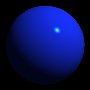
In order to limit the scope down to a manageable size I've not implemented multiple objects or sphere transformations (shearing, rotation, etc.). In the case of transformations I don't think they would present much further work, partly due to the fact that J natively provides an operation to invert a matrix (%.).

Thoughts

Developing all of this in J proved to be an impressively interactive experience. The combination of a pretty good console and editor meant trying things out iteratively and debugging errors on the fly was nearly painless. Paired with a few helpful features of the J editor like context-sensitive help meant I could jump to the documentation where there are plenty of examples.

Frankly I've been surprised at how much I like J; when I first learned some Klong and later read about K I thought that J looked off-putting for the "needlessly weird" syntax and went so far as to try out APL which I reasoned had more cause for weird syntax owing to its history. Finally digging into J some more reveals a lot of thought has gone into the design of the language and things feel very...regular? It is hard to explain exactly, but I keep finding myself surprised when things just work. I'll type something out, feed some test input, make an amendment and it'll be done. No weird edge cases, no confusing discrepancies, it takes a little while to get up to speed but the learning curve has not been so steep as I imagined.

I should also mention, it is fast. I've written a very similar ray tracer in Common Lisp (which I won't claim to be any good at, but certainly have at least as much experience in) and without optimizing anything in either implementation J is performing around 5 times as fast. While it isn't very fair to CL or indicative of what can be done in the language it does seem telling that a fast solution is more apparent in J, at least to this novice.

The full program is here.