I spent some time sitting on planes recently and got to thinking about computer vision and image manipulation, as one does. In an effort to discover for myself the fundamentals of the field I set about working out how to "derive" image contours in the most naive way possible.
I was unfamiliar with much of the terminology when I worked this all out, but some recent reading has led me to the following general definitions:
Given an arbitrary matrix that I've transcribed out of my in-flight notes (written here in Klong):
        example::[
[0 0 0 0 0 0 0 0 0 0]
[0 1 1 1 0 0 0 0 0 0]
[0 1 1 1 0 1 1 1 0 0]
[0 1 1 1 1 1 1 1 0 0]
[0 1 1 1 1 1 1 1 0 0]
[0 1 1 1 1 1 1 1 0 0]
[0 0 1 1 1 1 0 0 1 0]
[0 1 1 1 1 1 0 0 1 0]
[0 1 1 0 0 0 0 0 1 0]
[0 0 0 0 0 0 0 0 0 0]]
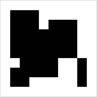
You can better picture the occupancy like so:
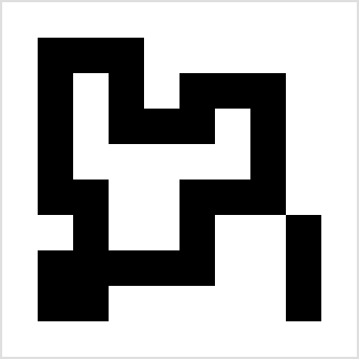
Where contours around these shapes would look like this:
Although I did not realize it at the time, I had already developed much of what I needed when I wrote my game of life implementation in Klong. In my defense, I was trying to "reverse engineer" the fundamentals of image processing on paper, so I hadn't quite made the connection to my own prior work.
I can (re)define the same move verb from my Game of Life that takes
a lateral (x), vertical (y) and starting matrix (z):
        move::{[a b]; a::x; b::y; {a:+x}({+b:++x}(z))}
:triad
Applying a move over shifts -1, 0, and 1 in both the vertical an
horizontal directions is accomplished with the verb neighbors (also
defined previously):
        neighbors::{[a]; a::x; +/,/{[b]; b::x; move(b;;a)'[-1 0 1]}'[-1 0 1]}
:monad
The result of such a "neighbor search" is actually more information than I need:
        neighbors(example)
 1 2 3 2 1 0 0 0 0 0
 2 4 6 4 3 2 3 2 1 0
 3 6 9 7 6 5 6 4 2 0
 3 6 9 8 8 8 9 6 3 0
 3 6 9 9 9 9 9 6 3 0
 2 5 8 9 9 8 7 5 3 1
 2 5 8 9 9 7 5 4 3 2
 2 5 7 7 6 4 2 3 3 3
 2 4 5 4 3 2 1 2 2 2
 1 2 2 1 0 0 0 1 1 1
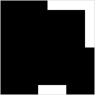
Rather than a count of occupied points I really only need a boolean,
so I'll apply logical negation (~) twice over the matrix, which
gives both the current occupancy and those points neighboring:
        ~~neighbors(example)
 1 1 1 1 1 0 0 0 0 0
 1 1 1 1 1 1 1 1 1 0
 1 1 1 1 1 1 1 1 1 0
 1 1 1 1 1 1 1 1 1 0
 1 1 1 1 1 1 1 1 1 0
 1 1 1 1 1 1 1 1 1 1
 1 1 1 1 1 1 1 1 1 1
 1 1 1 1 1 1 1 1 1 1
 1 1 1 1 1 1 1 1 1 1
 1 1 1 1 0 0 0 1 1 1
It is admittedly, not much to look at with so many points neighboring.
If the original matrix is removed then what is left are those points bordering the orignal:
        border::(~~neighbors(example))-example
 1 1 1 1 1 0 0 0 0 0
 1 0 0 0 1 1 1 1 1 0
 1 0 0 0 1 0 0 0 1 0
 1 0 0 0 0 0 0 0 1 0
 1 0 0 0 0 0 0 0 1 0
 1 0 0 0 0 0 0 0 1 1
 1 1 0 0 0 0 1 1 0 1
 1 0 0 0 0 0 1 1 0 1
 1 0 0 1 1 1 1 1 0 1
 1 1 1 1 0 0 0 1 1 1
I had actually stopped at this point, thinking I was "done" and had defined a contour for a given matrix, but upon reading this page I realized I hadn't quite satisfied the normal definition of a contour by extending the bounds of the original matrix.
With that in mind I tried applying a second variation of the
"neighbor" algorithm but rather than taking a sum I take a maximum of
the neighboring points by applying "max" (|) over each of the 9
matrices resulting from rotation in -1, 0, and 1:
        MaxN::{[a]; a::x; |/,/{[b]; b::x; move(b;;a)'[-1 0 1]}'[-1 0 1]}
:monad
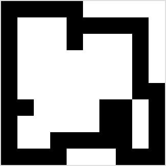
This successfully zeroes out the interior points but leaves many points neighboring the border points with values where there should be none. I remove these by applying a logical-and with the max-matrix and the original:
        MaxN(border)&example
 0 0 0 0 0 0 0 0 0 0
 0 1 1 1 0 0 0 0 0 0
 0 1 0 1 0 1 1 1 0 0
 0 1 0 1 1 1 0 1 0 0
 0 1 0 0 0 0 0 1 0 0
 0 1 1 0 0 1 1 1 0 0
 0 0 1 0 0 1 0 0 1 0
 0 1 1 1 1 1 0 0 1 0
 0 1 1 0 0 0 0 0 1 0
 0 0 0 0 0 0 0 0 0 0
Satisfied with my results I didn't think too much further about it until today, when reading about Moore Neighborhood on Wikipedia. I found out that a generalization of the same problem "was a great challenge for most analysts of the 18th century". Always feels good to discover I'm thinking like the experts, only a few hundred years behind. The algorithm described works bottom to top and circles occupied points clockwise, which is very similar to the 9 rotational matrices I implemented. I think the algorithm outlined is more efficient, but perhaps more fiddly as well.
I think I'm gradually working my way up to applying these techniques through matrix convolution like I've been reading about with the Sobel operator or the Prewitt operator. I think by performing the boundary-checking through what I term a "neighbor" search (checking those 8 points surrounding a pixel) I am actually approaching the kind of gradient descent techniques that are more commonly used. Personally, it helps me to understand first the more mechanical approach before the revelation of "this is a single matrix operation!".
In an effort to ease some of this development, specifically generating
the images above, I defined a helper function to output the images in
PBM format (though this does require the function pm, print matrix,
provided in the Klong book):
        pbm::{.p("P1"); pm(,1:+^x); pm(x)}
:monad
All pbm does is supply header information, P1 is for bitmap images
using ASCII 1s and 0s, on the second line I am printing (.p) the
shape of the rotated argument matrix x, then nesting it to create an
array of one element, the array of shape. This last bit is a minor
oddity to match the API of the matrix printing verb. Finally I print
the matrix itself, formatted into a "pretty" layout:
        pbm(example)
P1
 10 10
 0 0 0 0 0 0 0 0 0 0
 0 1 1 1 0 0 0 0 0 0
 0 1 1 1 0 1 1 1 0 0
 0 1 1 1 1 1 1 1 0 0
 0 1 1 1 1 1 1 1 0 0
 0 1 1 1 1 1 1 1 0 0
 0 0 1 1 1 1 0 0 1 0
 0 1 1 1 1 1 0 0 1 0
 0 1 1 0 0 0 0 0 1 0
 0 0 0 0 0 0 0 0 0 0
Of course, the images I am generating are 10 pixels square, while the pictures above are much larger. The trick to this is through imagemagick, by scaling up the image rather than resizing, there is no blurring to the larger image. I also converted to PNG so that browsers can display them.
convert sample.pbm -scale 3200% larger-sample.png